Access to High-Quality Data With Error Detection
Classical computing has been transformed by the enormous volumes of high-quality data readily available for advanced applications in machine learning (ML), artificial intelligence (AI), and related technologies. Complex patterns of text, images, videos that are fundamentally in the form of classical bits (0s and 1s) feed the models that we rely on to perform increasingly sophisticated tasks.
At the same time, quantum computing is advancing like never before. Exciting announcements about new applications, control capabilities, and technological demonstrations are highlighting how the field is moving full speed toward delivering something of commercial value to the world. This too will bring transformational change to computing as we know it.
So, is there an intersection between quantum, ML, and AI today? On the software and applications level, certainly – from managing system calibration at scale, to error correction decoders, and more. On the hardware level, with existing quantum processing units (QPUs), there’s still a missing element. We know that error-corrected systems can provide high-quality data as inputs to ML or AI applications, but those aren’t online yet. Is there anything today?
Near-term conventional quantum computing systems (of the NISQ variety), which return measurement results consisting of 0s and 1s only, fall prey to standard “decoherence”, where silent errors creep in like fog. These errors degrade the final result, and users have no way to identify or back out where the error occurred. The lack of error correction on these systems means that they are solely limited by the performance of their constituent physical qubits.
This is where Quantum Circuits comes in.
The Dual-Rail Cavity Qubit (DRQ) is a high-performance qubit developed by Quantum Circuits that introduces built-in error detection at the qubit level. At its center is a new type of measurement – the * – which means an error was measured. There are three possible measurements of the qubit in the DRQ-based QPU: 0, 1 and *, where * means the qubit is in the error state at the end of the calculation.
The * is a new, high-quality piece of data. It reflects the dominant source of error in the system, which is called an erasure. Unlike other systems, where silent errors dominate and degrade the result quality in unknown ways, our systems send up a flare when an error is encountered. These events can be detected, recorded, and provide information that can be used in multiple ways to produce significantly better results.
The extra data containing *s is useful. One can just discard it and boost the performance of the quantum application. However, it comprises a data record in its own right. It contains information, however imperfect, about what happened to the qubits in an algorithm, and it should be leveraged rather than ignored. As we’ll see in the following chapters, such information can be in the form of rich patterns of many data records, which together point to directions about how to improve algorithm performance.
This is where the intersection with Machine Learning occurs. Over the next two chapters, we will go through exciting, illustrative results that motivate how a DRQ-based QPU can yield new insights through such patterns and relationships between measurement records with and without detected errors.
This indeed can be thought of as error mitigation. However, error detection is very efficient. In real time, the QPU is returning a record of error data – the new result * introduced earlier – that you can custom process any way you wish. This is an evolution beyond NISQ. And it is part of our roadmap to deliver systems that expand the space of what’s possible.
Identifying Patterns with Unsupervised Machine Learning
With additional data available to us about errors in the computation, we can analyze QPU outputs in multiple ways to extract insights from our error-detected quantum computers. The use of machine learning is just one promising approach among many. Unsupervised machine learning allows us to discover hidden patterns in the data without preconceived ideas about what we might find. The patterns identified through this type of exploration can inform subsequent supervised machine learning efforts, offering a systematic approach to understanding how to take advantage of valuable quantum error information.
The input to the analysis is data we acquired from our Aqumen Seeker QPU, built on our high-performance Dual-Rail Cavity Qubit architecture. We ran an 8-qubit Bernstein-Vazirani (BV) and a 5-qubit Grover search algorithm. These examples have the advantage of returning a single bit string in the ideal case, simplifying the analysis. Looking ahead, we will also include data from algorithms that measure arbitrary states. We chose to run both BV and Grover because the former is a simple starter example to get a feel for how the error detection returns data, and Grover because it is a non-trivial algorithm that may contain some interesting error data records and patterns. We also ran Grover on a different, non-Quantum Circuits superconducting QPU to demonstrate what one sees when obtaining only 0s and 1s without error detection.
We first start by describing a key plot type that will be used to visualize the data from our QPU. This is called the isomap. An isomap is a clever way to take complex data with hundreds or thousands of dimensions and create simple 2D maps that you can look at and understand. The key insight is that it depicts data “geographically”, like on a map, and distances between data points represent relationships between those data points. The closer they are, the more related, the farther they are, the less. This approach reveals hidden patterns and clusters in the data that would otherwise be difficult to identify, making it especially useful for discovering natural groupings and patterns that we’ll be applying to the ML example.
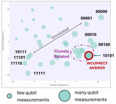
An example of an isomap is shown in Figure 1. It depicts the results from a non-Quantum Circuits superconducting QPU running Grover’s search on five qubits. Several features are highlighted. Each circle represents the number of counts measured out of the 1,000 shots acquired in that particular run. The smaller the circle, the fewer the counts. Circles that are close to one another tend to have measurement strings, or patterns, that are closely related, such as 11110 and 11101. When they are far apart, they tend to be unrelated, such as 11111 and 00000. The circle outlined in red contains the largest number of counts, and yet 10101 is the incorrect answer in this particular run of Grover’s search. This is the effect of the silent errors – decoherence – degrading the final result.
There doesn’t seem to be much in the way of a clear pattern in the isomap. Perhaps some correlations do exist, but many tools to understand any existing subtle relationships already provide predictive insight as to how and why QPUs return noisy data. This is not the high-quality data we’re looking for.
Now, let’s look at an example of a Quantum Circuits QPU run of BV with error detection turned on, using eight qubits. The data is shown in Figure 2.
To underscore the unique qualities of a data sample with detected errors, we adjusted the algorithm to include approximately 100 more single and two-qubit gates than required, while keeping it logically equivalent. We wanted to increase the number of errors so we could more easily inspect the patterns our isomaps were producing.
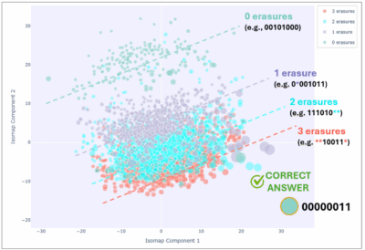
There is a lot to absorb, so let’s walk through it. The BV algorithm concludes with a measurement on each of the eight qubits, so the final measurement result could look like 00101000. However, each of these eight qubits could run into an error – or so-called “erasure” – throughout the course of the algorithm. For example, this could be the second qubit. The measurement record could therefore be: 0*001011. The same pattern repeats for two errors, three, etc. The isomap is the same as before, but this time it has four categories of colored points: green (no detected errors), purple (one detected error), cyan (two detected errors), and red (three detected errors). Greater error numbers are omitted for clarity.
The difference between this result and the first isomap is stark. The correct answer, at the bottom right, is prominent and situated far away from the remaining majority of smaller green circles towards the top left. This is one of the huge advantages of having a system in which the dominant error is not silent – picking out erasures via error detection not just enhances the right answer, in this case it makes it possible to even identify it.
Next, although the erasures are indeed errors, unlike in the first plot, they are not scattered haphazardly. There are clear bands, visually marked by the dotted lines, leading from the 3-erasure case up to the 0-erasure case. There are even larger 1-erasure circles that lie in an area dominated by the 3-erasure case, geographically closer to the correct answer and indicating potentially an important and noteworthy relationship.
This is the kind of data we want to be looking at. It inspires us to seek whether the patterns are telling us something more than just errors occurred. We start to treat this not as just “errors”, but as new “data” that contains information about the trajectory our qubit took on its way to some final answer. Are there relationships between these patterns and the final answer? What about the size of each circle – is that relevant? What do we see if we execute the same algorithm but for different inputs?
In the next chapter next week, we dig into a more a complex example – Grover’s algorithm – and uncover a rich tapestry of patterns. As we’ll see, it motivates novel techniques in supervised ML with Dual-Rail Cavity Qubit QPUs.